A simple, yet powerful concept used during data analysis that
categorizes the data into different buckets/bins. One important point to
remember is that “binning” and “clustering” are not the same and vary considerably in logic and implementation. Binning as a method of data pre-processing. Data binning (or bucketing) groups data in bins (or buckets), in the sense that it replaces values contained into a small interval with a single representative value for that interval. Sometimes binning improves accuracy in predictive models.
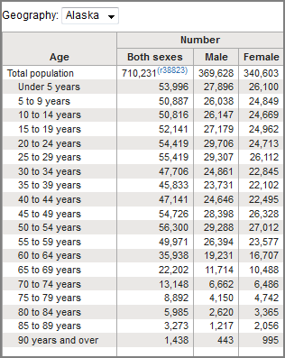
Image of binning census data by age group -

Sometimes, binning can improve accuracy of the predictive models. In addition, sometimes we use data binning to group a set of numerical values into a smaller number of bins to have a better understanding of the data distribution.
As example, “a automobile price” is an attribute range from 5,000 to 45,500.
Using binning, we categorize the price into three bins: low price, medium price, and high
prices. In the actual automobile dataset, ”price" is a numerical variable ranging from 5188 to 45400,
it has 201 unique values. We can categorize them into 3 bins: low, medium, and high-priced cars.
In Python we can easily implement the binning: We would like 3 bins of equal binwidth, so
we need 4 numbers as dividers that are equal distance apart.
1) First we use the numpy function “linspace” to return the array “bins” that contains
4 equally spaced numbers over the specified interval of the price. 2)We create a list “group_names “ that contains the different bin names.
3) We use the pandas function ”cut” to segment and sort the data values into bins.
We can then use histograms to visualize the distribution of the data after they’ve been
divided into bins. This is sample histogram that we plotted based on the binning that we applied in the price feature. From the histogram plot, it is clear that most cars have a low price, and only very few cars have high price.
Another example of binning employee data by salary.


No comments:
Post a Comment